Grid
At a glance
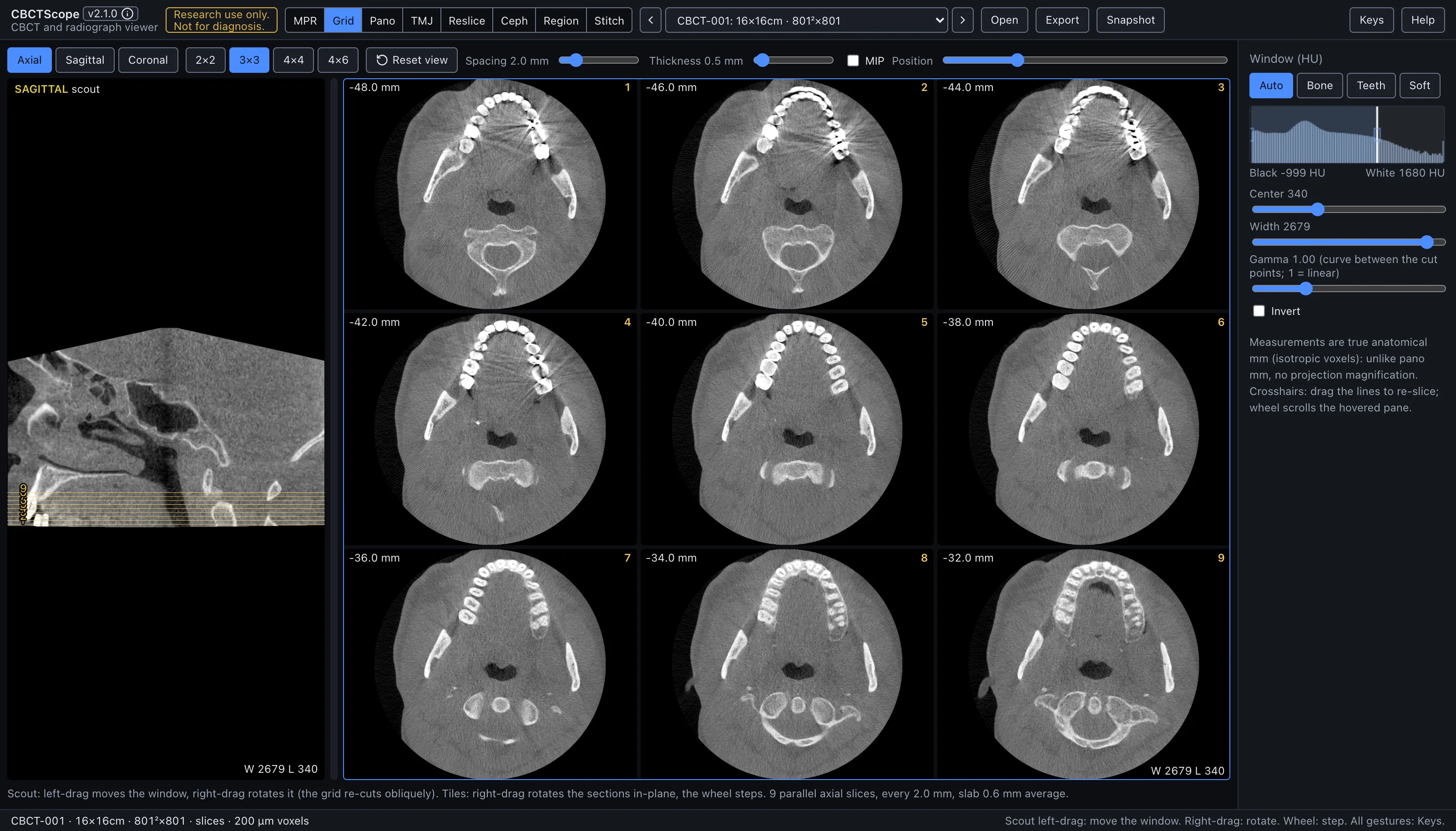
- What the view shows: show this whole region slice by slice at a glance, at a chosen spacing and any angle, the way a printed multi-slice sheet would.
- Start: pick the plane and a grid size, set the window, then drag the section window over the region on the scout and set the spacing so the stack covers it.
- Three gestures: on the scout, left-drag moves the section window and right-drag rotates the stack through the anatomy; the wheel, anywhere in the mode, steps the window by one spacing. The Keys card lists every gesture of the mode.
- Leave it for: measurements, annotations, and saved views, which live in MPR.
What this mode is for
Grid shows many parallel slices of one stack on one screen: a chosen number of images at a chosen spacing and slab thickness, cut along the axial, sagittal, or coronal direction, or along any oblique direction you rotate into. It answers the survey question: "show me this whole region, slice by slice, at a glance," the way a printed multi-slice sheet would, with the added ability to re-angle the entire stack through the anatomy.
Gestures
| Gesture | Where | Action |
|---|---|---|
| Left-drag or click | scout | Grab the section window and move it |
| Right-drag | scout | Rotate the scout image itself: the section lines stay put on screen while the anatomy turns under them, and the grid re-cuts obliquely through the rotated anatomy, with a live degree chip during the drag |
| Wheel | anywhere in the mode | Step the whole window by one spacing unit |
| Double-click a slider | controls | Reset it |
The tiles themselves are display-only.
The controls
| Control | Options or range | What it does |
|---|---|---|
| Plane | Axial, Sagittal, Coronal | The initial cutting direction. Switching planes straightens a rotated stack (announced briefly in the on-screen chip) but keeps your window position along the new axis; re-clicking the already-active plane does nothing, so a tuned oblique cannot be wiped by a stray click. The Reset view button straightens in place. |
| Grid size | 2×2, 3×3, 4×4, 4×6 | The tiles on screen. The selected plane and grid size are solid blue. Each tile is labeled with its offset in mm from the stack center and a tile number that matches the numbered section lines on the scout; the window reads bottom right of the scout and of the last tile, and the pane that takes the wheel carries a thin blue frame. |
| Spacing | 0.5 to 10 mm | The distance between consecutive slices in the stack. |
| Thickness | 0.1 to 10 mm | The slab averaged into each slice; the MIP checkbox takes the brightest voxel across the slab instead of the average. |
| Reset view | button | Back to the straight orthogonal stack after any rotation. |
| Position | slider | Moves the whole slice window along the stack normal. |
| Scout pane | left | The control surface: the perpendicular reference view (a sagittal scout for an axial grid, an axial scout otherwise) with one numbered line per tile. |
| Window | shared sidebar | The shared Window (HU) panel applies here, including the presets, the histogram cut lines, center and width, gamma, and invert. |
| Note | under the grid | Restates the current geometry: how many parallel slices, at what spacing, with what slab, averaged or MIP. |
A reading workflow
- Pick the plane that matches the question, and a grid size that fits the extent of the region: a small grid for a focused area, 4x6 for a long sweep.
- Set the window before reading: Bone or Teeth for skeletal review, Soft for the soft-tissue survey.
- On the scout, drag the section window over the region of interest, then set spacing so the stack covers it edge to edge.
- Choose spacing no larger than the smallest structure you want to be sure of catching, or step the window with the wheel so consecutive positions overlap.
- If the anatomy runs oblique to the standard planes, right-drag on the scout until the stack cuts along it, and use Reset view to return.
- Read the tiles in numbered order and cross-check any tile against the scout: the numbered line shows exactly where that slice cuts.
- Keep the slab thin for fine detail; use a thicker slab, or MIP, when continuity of a high-density structure across noise matters more than sharpness.
- For the record, switch to MPR and use its snapshot and measurement tools at the position identified here.
Over MCP
open_scan, list_volumes, select_volume, set_view_mode (mode grid), and
set_window_level apply; snapshot captures the scout and all tiles as laid out.
navigate_slice moves the window centre along the grid's plane: index is the centre
slice in the pane count (unrotated grid), delta steps whole grid spacings like the
wheel, and pane switches the plane. viewer_state reports the plane, the centre slice,
the tile count and spacing, and whether the grid is rotated (then the index runs along the
oblique normal). A plain reset_view has no camera to reset in this mode; reset_view
with full: true still returns the shared window to its defaults. Example sequence:
set_view_mode to grid, set_window_level preset Bone, navigate_slice with
pane: "coronal" and an index, snapshot.
Limits
Grid is a survey surface, not a measurement surface: it has no calipers, no annotations, and no saved views; those live in MPR. Tiles cannot be individually windowed or zoomed. The stack geometry (count, spacing, thickness, rotation) is set with the on-screen controls only, not over MCP. CBCTScope is navigation and visualization only: no findings, no diagnoses. Research use only; not a medical device.